Mike Dusenberry
About
Nov 19, 2017
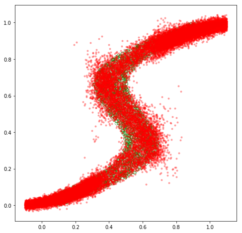
Mixture Density Networks
May 7, 2017
Research Paper: "Artificial neural networks: Predicting head CT findings in elderly patients presenting with minor head injury after a fall"
Jan 22, 2015
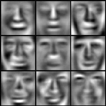
On Eigenfaces: Creating ghost-like images from a set of faces.
Jan 20, 2015
New Blog
Excited to start a new blog!